Studio Quickstart
f8pystudio is the visual graph editor for building, inspecting, deploying, and debugging Feel8 graphs.
This page is the first-stop user guide: it explains what the main window is for, how to place and wire nodes, where to configure them, and how to get from an empty canvas to a running graph without reading the full manual first.
Launch
If you are using a packaged release, launch the bundled f8pystudio app.
When working from the repository, prefer pixi:
pixi run -e default f8pystudio
For live discovery during development:
pixi run -e default python -m f8pystudio.main --discovery-live
Four Ideas To Keep In Mind
Before you start placing nodes, keep these distinctions clear:
Servicenodes represent real runtime services and appear in the deployed graph.Operatornodes usually run inside a host service such asf8.pyengine.UI / Visualizationnodes are mainly for local inspection and authoring-time interaction.- Edges come in three kinds:
Exec,Data, andState.
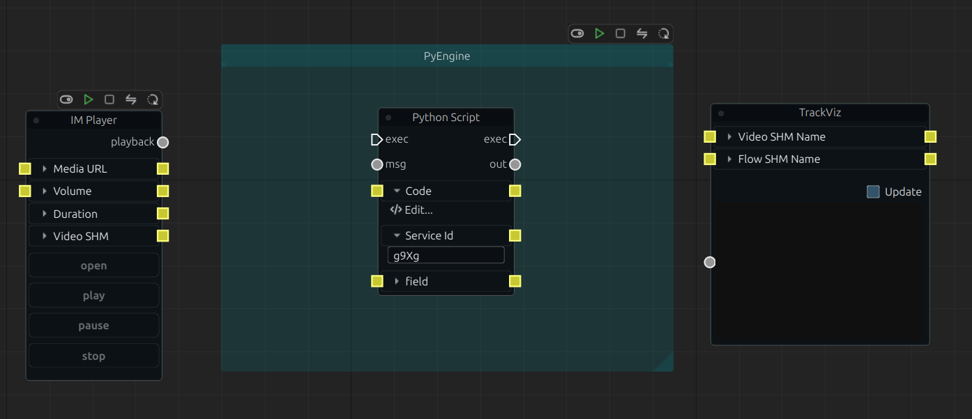
Most common first mistake
Many operator nodes require a valid Service Id. If an operator looks correctly wired but never runs, check the host binding first.
5-Minute Workflow
For a first graph, use this order:
- Place a host service such as
PyEngine. - Place your inputs, processing nodes, and visualizers.
- For every hosted operator, verify
Service Id. - Wire
Exec,Data, andStateedges with the intended meaning. - Select each important node and fill in required state fields in
Properties. - Save the project with
Ctrl+S. - Deploy with
F5. - Watch
Service MonitorandService Logsto confirm the graph is actually running.
A useful minimum setup is:
one host service + one operator + one visualization node
Reading The Main Window
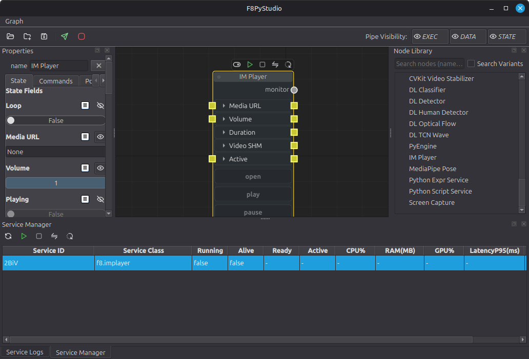
The main window is easiest to understand as five zones:
- Top toolbars: project actions, deploy/stop actions, edge visibility toggles, and asset cloud account access.
- Center canvas: the graph you are editing.
- Left
Propertiesdock: state fields, commands, ports, and node metadata for the current selection. - Right docks:
Node Library,Layers, andAI Assist. - Bottom docks:
Service LogsandService Monitor.
The key mental model is:
- The canvas is the editor view.
- Deployment compiles the canvas state into a runtime graph.
- Visual layout helps humans read the graph, but runtime behavior is defined by services, operators, state, and connections.
Start Here On A New Graph
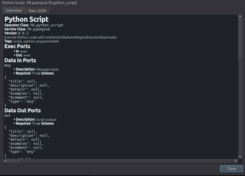
1. Node Library
Node Library is the fastest way to discover and place nodes.
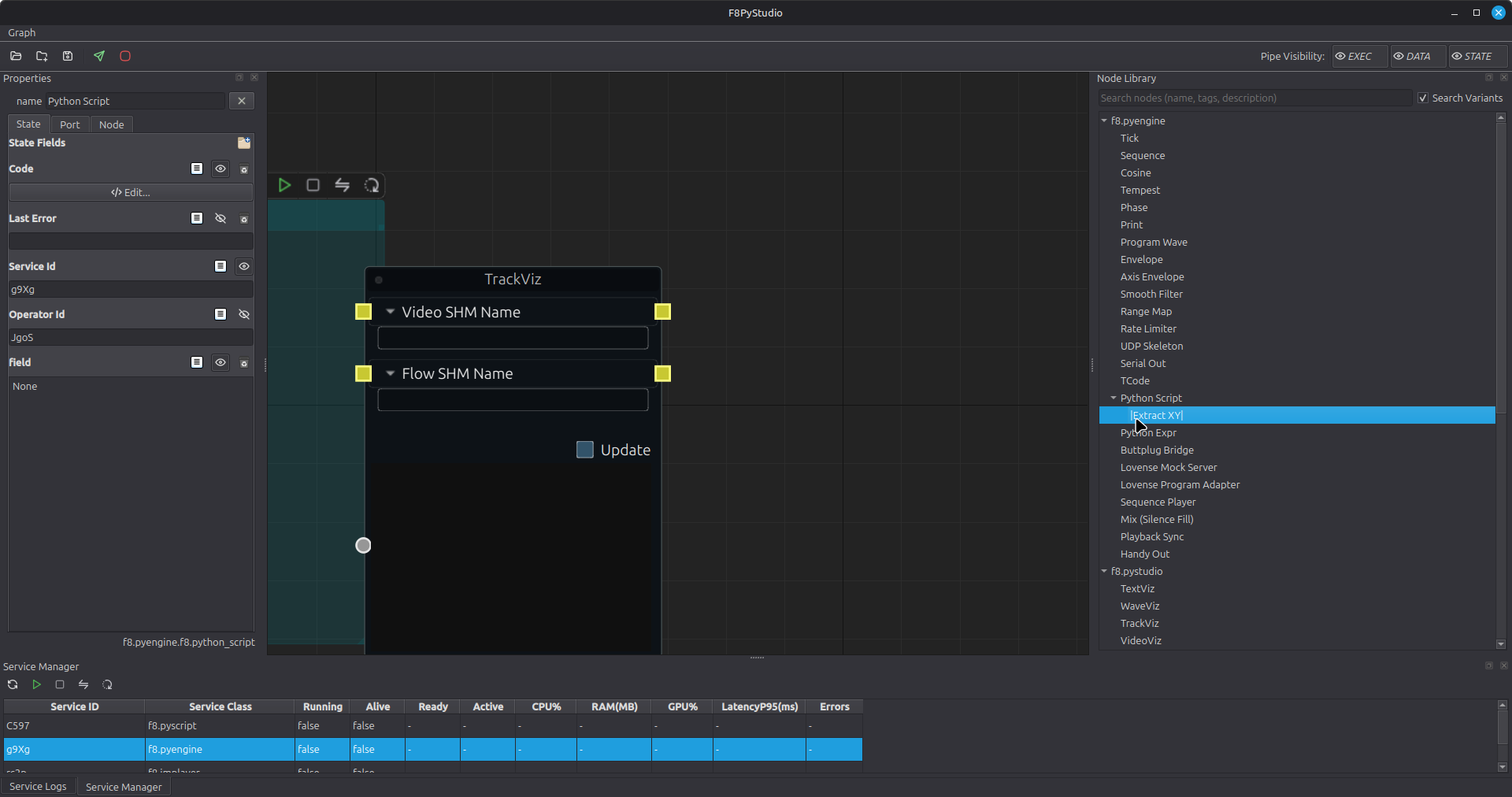
Typical usage:
- Search by name, tags, or description.
- Click a node entry.
- Click on the canvas to place it.
- Enable
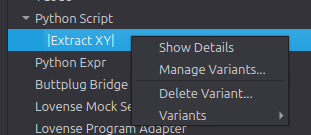
Search Variantsif you also want saved variants to appear in search results. - Right-click entries for details or variant actions.
2. Properties
Once a node is selected, most real work happens in Properties.
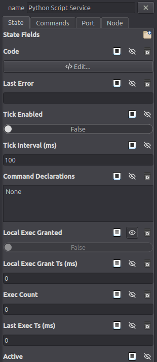
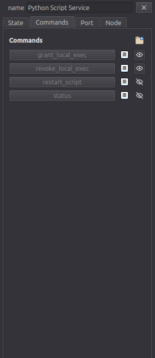
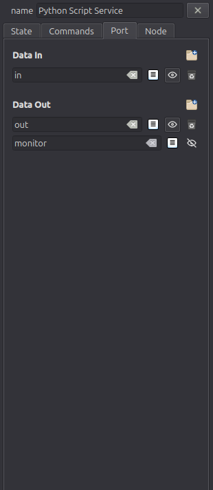
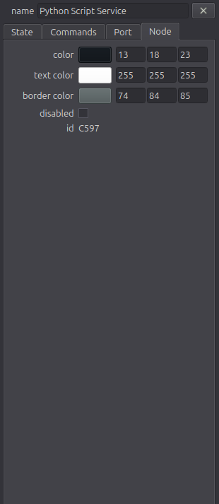
The most important tabs are:
State: node state, defaults, required flags, and inline visibility.Commands: callable commands and their parameters.Port: input/output port definitions and schemas.Node: labels, visuals, and layer membership.
Good habits:
- Define state and ports before writing expressions or script logic.
- Treat missing required fields as deploy blockers.
- If a state field becomes read-only, check whether it is currently driven by a state edge.
3. Service Toolbar States
Service nodes include a compact process toolbar. These states are worth learning early:
| Status | Screenshot | Meaning |
|---|---|---|
| Not Run | 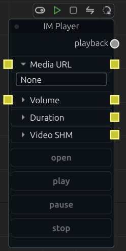 |
Process not started |
| Disabled | 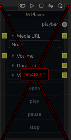 |
Excluded from compile and deploy |
| Running | 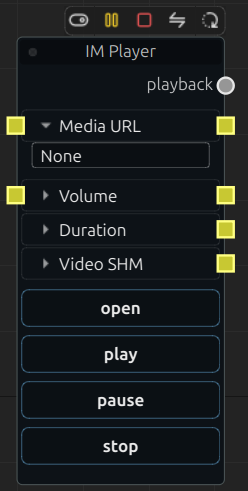 |
Process is alive |
| Paused | 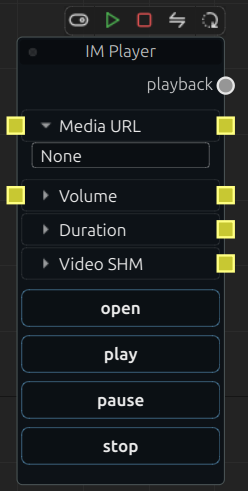 |
Process is alive but inactive |
Many early issues turn out to be service state issues rather than graph-shape issues.
The Most Useful Side Panels
Layers
Layers help organize larger graphs. Use them to group nodes by stage, scenario, or purpose, then show, hide, solo, reorder, and color-code those groups.
Use cases:
- separate capture, analysis, control, and visualization stages
- keep multiple scenario variants in one graph
- temporarily hide experimental branches without deleting them
Screenshot placeholder:
Layerspanel showingShow All,Reset to Defaults,Add Layer,Solo, color, and edit actions.
Service Monitor
After deployment, Service Monitor is the quickest health dashboard. It shows:
RunningAliveReadyActiveCPU%RAM(MB)GPU%LatencyP95(ms)Errors
It also gives row-level controls for:
- refresh
- start or activate
- stop
- deploy to one service
- restart and redeploy
Screenshot placeholder:
Service Monitorpanel with one or two service rows and the refresh/start/stop/deploy/restart buttons.
Service Logs
Service Logs are organized per service tab and are the first place to look for:
- deploy acceptance or rejection
- missing state fields
- runtime exceptions and tracebacks
- confirmation that a service is actively producing output
Tabs support clearing and saving logs, which is useful when isolating one failing service.
AI Assist
AI Assist is graph-aware rather than being a generic detached chat box. It can work from:
- the current node selection
- the current subgraph selection
- manually pinned graph context
Typical uses:
- explain a branch of the graph
- review configuration choices
- assist with code or schema drafting
- inspect the exact context being sent to the assistant
Screenshot placeholder:
AI Assistpanel with context usage, selected/pinned graph labels, pin/clear buttons, and the main chat area.
Components And Variants
Components Catalog
When you have a reusable subgraph, save it as a component with File -> Save As Component.
You can then reuse it through:
File -> Components CatalogFile -> Insert Component- canvas
Tabsearch entries such asComponent | ...
Use components for reusable graph structure.
Screenshot placeholder:
Components CatalogwithMine / Community / Installed, the entry list, and thePreview / Rawdetail pane.
Variant Catalog
Use variants when you want reusable presets for one node type rather than a whole subgraph.
Good examples:
- different visual styles for one visualization node
- different threshold sets for one processing node
- stable per-scenario parameter profiles
Open variants from the Node Library context menu or via Tools -> Variant Catalog.
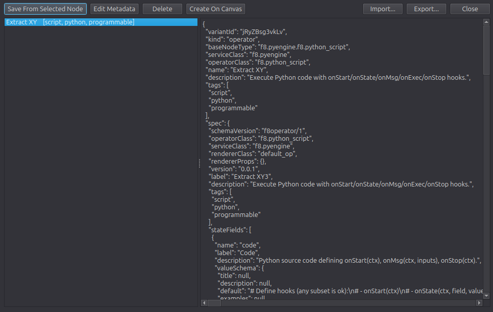
Rule of thumb:
- reusable structure ->
Component - reusable node preset ->
Variant
Asset Cloud Account
The account button in the upper-right toolbar is the asset cloud entry point. After signing in, component and variant browsers expose views such as:
MineCommunityInstalled
Those views are used for sync, sharing, subscription, import/export, and local-vs-remote management.
Project Saving And History
Studio now has local project storage and history, not just a single temporary session file.
The actions most users will care about are:
Ctrl+S: save projectCtrl+O: open projectCtrl+Shift+S: save asFile -> Project History: browse and restore earlier versionsFile -> Import Project JSONFile -> Export Project JSONFile -> Export Publish JSON
If Auto Save is enabled, Studio will continuously update the local stored project as you work.
If you want to inspect registered global shortcuts, open Tools -> Global Hotkeys.
Schema And Code Editors
Some nodes use richer editors than plain text inputs.
The schema editor helps define explicit contracts:
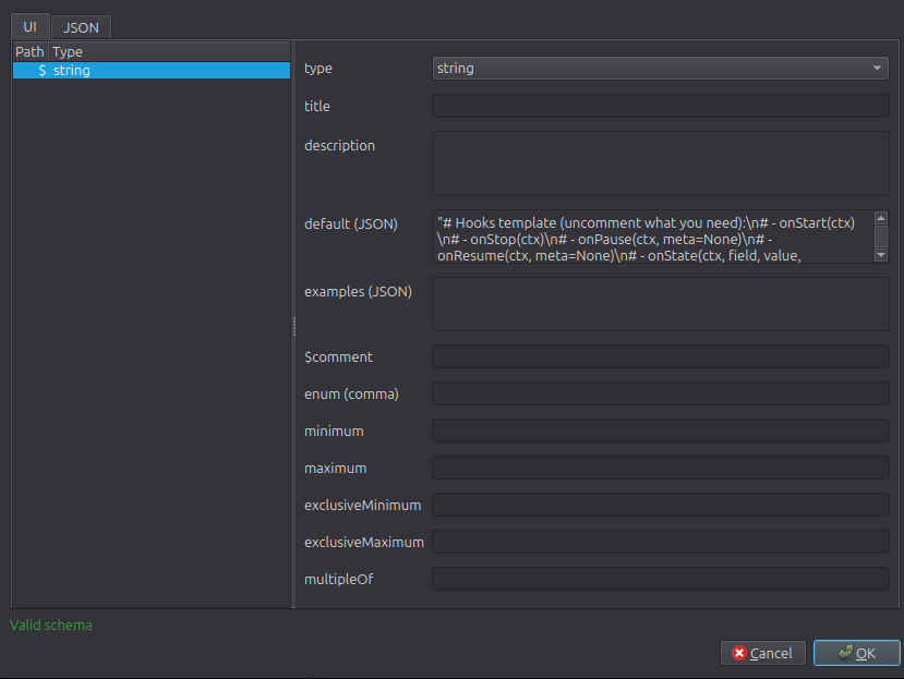
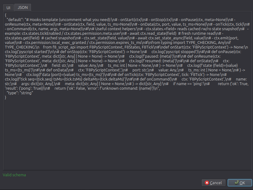
For code-heavy nodes, Studio provides a Monaco editor:
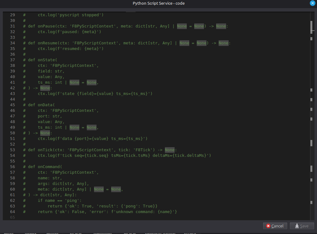
Common shortcuts:
Ctrl+S: saveCtrl+Q: closeCtrl+Space/Ctrl+J: completionCtrl+Shift+Space/Ctrl+Shift+J: parameter hintsEsc: close the suggestion popup
A Good Deploy Loop
Treat editing as a short loop:
- change nodes or wires
- verify
Properties - save with
Ctrl+S - deploy with
F5 - inspect
Service Monitor - inspect
Service Logs - restart only the failing service when possible
Helpful supporting features:
Auto SaveAuto DeployAuto ProxyPerformance OverlayEXEC / DATA / STATEvisibility toggles
Useful Shortcuts
| Shortcut | Action |
|---|---|
Tab |
Open node/component quick search |
Esc |
Cancel placement |
Delete / Backspace |
Delete selection |
Ctrl+S |
Save project |
Ctrl+O |
Open project |
Ctrl+Shift+S |
Save as |
F5 |
Deploy graph |
Shift+F5 |
Stop all services |
| Middle mouse drag | Pan canvas |
W/A/S/D or arrow keys |
Pan canvas |
Q/E or PageUp/PageDown |
Zoom |
Common First Problems
1. The graph looks wired, but an operator does not run
Check:
- whether
Service Idpoints to the correct host service - whether that service is actually
RunningandActive
2. Two ports refuse to connect
Common reasons:
- edge kind mismatch between
Exec,Data, andState - wrong direction
- schema or connection rule mismatch
3. Deploy is rejected
Check:
- required state fields
- disabled nodes
- missing hosts or invalid references
- explicit error lines in
Service Logs
4. The graph is getting too large to understand
Start using:
LayersComponentsVariantsNote/Backdrop
Those tools pay off early.